This note addresses the steps in the symmetrization technique in empirical process theory in probability. I will walk through each step and provide explanations. If you have some confusion and questions about this technique, like me, then this might be helpful to you! I encountered the argument perhaps 5 or 6 years ago, and I thought I knew what was going on. Until recently, I realized I missed something (especially the step  below), when I tried to use it in my own research.
Setup. Consider a finite function class of size  ,
,  where
where  is a set. We are given a series of independent random varaibles
  ,
,  , which take value in . Let
  . A typical quantity appeared in empirical process theory is
![\displaystyle \mathbb{E}\left [ \sup_{f\in \mathcal{F}} \frac{1}{n}\sum_{i=1}^n \left( f(X_i) - \mathbb{E}(f(X_i) \right) \right]. \ \ \ \ \ (1)](https://s0.wp.com/latex.php?latex=%5Cdisplaystyle+%5Cmathbb%7BE%7D%5Cleft+%5B+%5Csup_%7Bf%5Cin+%5Cmathcal%7BF%7D%7D+%5Cfrac%7B1%7D%7Bn%7D%5Csum_%7Bi%3D1%7D%5En+%5Cleft%28+f%28X_i%29+-+%5Cmathbb%7BE%7D%28f%28X_i%29+%5Cright%29+%5Cright%5D.+%5C+%5C+%5C+%5C+%5C+%281%29&bg=ffffff&fg=000000&s=0&c=20201002)
And we aim to upper bound it using the so-called Rademacher complexity (to be defined later).
The symmetrization argument. The symmetrization argument uses (1) an independent copy of  , denoted as
  , and (2)
  independent Rademacher random variables,
 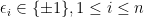 with
with 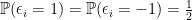 . Denote
  . Let us display the symmetrization argument:
![\displaystyle \begin{aligned} & \mathbb{E}\left [ \sup_{f\in \mathcal{F}} \frac{1}{n}\left( \sum_{i=1}^n f(X_i)- \mathbb{E}f(X_i) \right) \right] \\ \overset{(a)}{=} & \mathbb{E}\left [ \sup_{f\in \mathcal{F}} \frac{1}{n}\left( \sum_{i=1}^n f(X_i)- \mathbb{E}_{X_i'}f(X_i') \right) \right] \\ \overset{(b)}{ =} & \mathbb{E}\left [ \sup_{f\in \mathcal{F}} \frac{1}{n}\left( \sum_{i=1}^n \mathbb{E}_{X_i'}(f(X_i)-f(X_i')) \right) \right]\\ \overset{(c)}{\leq} & \mathbb{E}_{X,X'}\left [ \sup_{f\in \mathcal{F}} \frac{1}{n}\left( \sum_{i=1}^n (f(X_i)-f(X_i')) \right) \right]\\ \overset{(d)}{=} & \mathbb{E}_{X,X',\epsilon}\left [ \sup_{f\in \mathcal{F}} \frac{1}{n}\left( \sum_{i=1}^n \epsilon_i(f(X_i)-f(X_i')) \right) \right]\\ \overset{(e)}{=} & \mathbb{E}_{X,X',\epsilon}\left [ \sup_{f\in \mathcal{F}} \frac{1}{n}\left| \sum_{i=1}^n \epsilon_if(X_i) \right| \right]+ \mathbb{E}_{X,X',\epsilon}\left [ \sup_{f\in \mathcal{F}} \frac{1}{n}\left| \sum_{i=1}^n \epsilon_if(X_i') \right| \right]\\ \overset{(f)}{=} & 2 \mathbb{E}_{X,\epsilon}\left [ \sup_{f\in \mathcal{F}} \frac{1}{n}\left| \sum_{i=1}^n \epsilon_if(X_i) \right| \right]. \end{aligned} \ \ \ \ \ (2)](https://s0.wp.com/latex.php?latex=%5Cdisplaystyle+%5Cbegin%7Baligned%7D+%26+%5Cmathbb%7BE%7D%5Cleft+%5B+%5Csup_%7Bf%5Cin+%5Cmathcal%7BF%7D%7D+%5Cfrac%7B1%7D%7Bn%7D%5Cleft%28+%5Csum_%7Bi%3D1%7D%5En+f%28X_i%29-+%5Cmathbb%7BE%7Df%28X_i%29+%5Cright%29+%5Cright%5D+%5C%5C+%5Coverset%7B%28a%29%7D%7B%3D%7D+%26+%5Cmathbb%7BE%7D%5Cleft+%5B+%5Csup_%7Bf%5Cin+%5Cmathcal%7BF%7D%7D+%5Cfrac%7B1%7D%7Bn%7D%5Cleft%28+%5Csum_%7Bi%3D1%7D%5En+f%28X_i%29-+%5Cmathbb%7BE%7D_%7BX_i%27%7Df%28X_i%27%29+%5Cright%29+%5Cright%5D+%5C%5C+%5Coverset%7B%28b%29%7D%7B+%3D%7D+%26+%5Cmathbb%7BE%7D%5Cleft+%5B+%5Csup_%7Bf%5Cin+%5Cmathcal%7BF%7D%7D+%5Cfrac%7B1%7D%7Bn%7D%5Cleft%28+%5Csum_%7Bi%3D1%7D%5En+%5Cmathbb%7BE%7D_%7BX_i%27%7D%28f%28X_i%29-f%28X_i%27%29%29+%5Cright%29+%5Cright%5D%5C%5C+%5Coverset%7B%28c%29%7D%7B%5Cleq%7D+%26+%5Cmathbb%7BE%7D_%7BX%2CX%27%7D%5Cleft+%5B+%5Csup_%7Bf%5Cin+%5Cmathcal%7BF%7D%7D+%5Cfrac%7B1%7D%7Bn%7D%5Cleft%28+%5Csum_%7Bi%3D1%7D%5En+%28f%28X_i%29-f%28X_i%27%29%29+%5Cright%29+%5Cright%5D%5C%5C+%5Coverset%7B%28d%29%7D%7B%3D%7D+%26+%5Cmathbb%7BE%7D_%7BX%2CX%27%2C%5Cepsilon%7D%5Cleft+%5B+%5Csup_%7Bf%5Cin+%5Cmathcal%7BF%7D%7D+%5Cfrac%7B1%7D%7Bn%7D%5Cleft%28+%5Csum_%7Bi%3D1%7D%5En+%5Cepsilon_i%28f%28X_i%29-f%28X_i%27%29%29+%5Cright%29+%5Cright%5D%5C%5C+%5Coverset%7B%28e%29%7D%7B%3D%7D+%26+%5Cmathbb%7BE%7D_%7BX%2CX%27%2C%5Cepsilon%7D%5Cleft+%5B+%5Csup_%7Bf%5Cin+%5Cmathcal%7BF%7D%7D+%5Cfrac%7B1%7D%7Bn%7D%5Cleft%7C+%5Csum_%7Bi%3D1%7D%5En+%5Cepsilon_if%28X_i%29+%5Cright%7C+%5Cright%5D%2B+%5Cmathbb%7BE%7D_%7BX%2CX%27%2C%5Cepsilon%7D%5Cleft+%5B+%5Csup_%7Bf%5Cin+%5Cmathcal%7BF%7D%7D+%5Cfrac%7B1%7D%7Bn%7D%5Cleft%7C+%5Csum_%7Bi%3D1%7D%5En+%5Cepsilon_if%28X_i%27%29+%5Cright%7C+%5Cright%5D%5C%5C+%5Coverset%7B%28f%29%7D%7B%3D%7D+%26+2+%5Cmathbb%7BE%7D_%7BX%2C%5Cepsilon%7D%5Cleft+%5B+%5Csup_%7Bf%5Cin+%5Cmathcal%7BF%7D%7D+%5Cfrac%7B1%7D%7Bn%7D%5Cleft%7C+%5Csum_%7Bi%3D1%7D%5En+%5Cepsilon_if%28X_i%29+%5Cright%7C+%5Cright%5D.+%5Cend%7Baligned%7D+%5C+%5C+%5C+%5C+%5C+%282%29&bg=ffffff&fg=000000&s=0&c=20201002)
The last quantity ![{ \mathbb{E}_{X,X',\epsilon}\left [ \sup_{f\in \mathcal{F}} \frac{1}{n}\left| \sum_{i=1}^n \epsilon_if(X_i) \right| \right]}](https://s0.wp.com/latex.php?latex=%7B+%5Cmathbb%7BE%7D_%7BX%2CX%27%2C%5Cepsilon%7D%5Cleft+%5B+%5Csup_%7Bf%5Cin+%5Cmathcal%7BF%7D%7D+%5Cfrac%7B1%7D%7Bn%7D%5Cleft%7C+%5Csum_%7Bi%3D1%7D%5En+%5Cepsilon_if%28X_i%29+%5Cright%7C+%5Cright%5D%7D&bg=ffffff&fg=000000&s=0&c=20201002) is called the Rademacher complexity of
is called the Rademacher complexity of  w.r.t. . In step
  and
and  , we uses the fact that and has the same distribution. In step
  , we use the fact that and are independent so that we could take the expectation w.r.t. first (or consider
 ![{\mathbb{E}_{X'}[\cdot]}](https://s0.wp.com/latex.php?latex=%7B%5Cmathbb%7BE%7D_%7BX%27%7D%5B%5Ccdot%5D%7D&bg=ffffff&fg=000000&s=0&c=20201002) as
as ![{\mathbb{E}[ \cdot \mid X]}](https://s0.wp.com/latex.php?latex=%7B%5Cmathbb%7BE%7D%5B+%5Ccdot+%5Cmid+X%5D%7D&bg=ffffff&fg=000000&s=0&c=20201002) ). In step
). In step  , we use the triangle inequality. Next, we explain the steps
  and .
and .
Step . Here in the step , we use the fact that for each  , we have
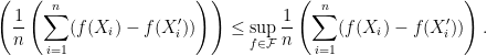
Taking the expectation over gives

After taking a superium over the left-hand side of the above over first and then taking an expectation over , we conclude the step .
Step . Step looks puzzling (to me) at first. A naive reasoning of is that  has the same distribution as
  . I was not convinced by this argument since we are taking a superium over .
Denote “equal in distribution” as  . The things we are (or I am) missing is that there are many s in . Hence, knowing that for each ,

is not enough. Let us first assume  is fixed. What we really need is to ensure that for any fixed , the joint distributions of the following two are the same,
![\displaystyle [f_j(X_i)-f_j(X_i')]_{1\leq i\leq n,1\leq j\leq m} \overset{\text{d}}{=} \left[\epsilon_i \left(f_j(X_i)-f_j(X_i')\right)\right]_{1\leq i\leq n,1\leq j\leq m}. \ \ \ \ \ (3)](https://s0.wp.com/latex.php?latex=%5Cdisplaystyle+%5Bf_j%28X_i%29-f_j%28X_i%27%29%5D_%7B1%5Cleq+i%5Cleq+n%2C1%5Cleq+j%5Cleq+m%7D+%5Coverset%7B%5Ctext%7Bd%7D%7D%7B%3D%7D+%5Cleft%5B%5Cepsilon_i+%5Cleft%28f_j%28X_i%29-f_j%28X_i%27%29%5Cright%29%5Cright%5D_%7B1%5Cleq+i%5Cleq+n%2C1%5Cleq+j%5Cleq+m%7D.+%5C+%5C+%5C+%5C+%5C+%283%29&bg=ffffff&fg=000000&s=0&c=20201002)
To argue (3), first, for each  , we have
![\displaystyle [f_j(X_i) - f_j(X_i')]_{j=1}^m \overset{\text{d}}{=} [\epsilon_i (f_j(X_i) - f_j(X_i'))]_{j=1}^m,](https://s0.wp.com/latex.php?latex=%5Cdisplaystyle+%5Bf_j%28X_i%29+-+f_j%28X_i%27%29%5D_%7Bj%3D1%7D%5Em+%5Coverset%7B%5Ctext%7Bd%7D%7D%7B%3D%7D+%5B%5Cepsilon_i+%28f_j%28X_i%29+-+f_j%28X_i%27%29%29%5D_%7Bj%3D1%7D%5Em%2C+&bg=ffffff&fg=000000&s=0&c=20201002)
by noting that ![[\epsilon_i (f_j(X_i) - f_j(X_i'))]_{j=1}^m = \epsilon_i [(f_j(X_i) - f_j(X_i'))]_{j=1}^m.](https://s0.wp.com/latex.php?latex=%5B%5Cepsilon_i+%28f_j%28X_i%29+-+f_j%28X_i%27%29%29%5D_%7Bj%3D1%7D%5Em+%3D+%5Cepsilon_i+%5B%28f_j%28X_i%29+-+f_j%28X_i%27%29%29%5D_%7Bj%3D1%7D%5Em.+&bg=ffffff&fg=000000&s=0&c=20201002) Hence, because of independence of
Hence, because of independence of  , we know that
![\displaystyle [[f_j(X_i)-f_j(X_i')]_{1\leq j\leq m}]_{1\leq i\leq n} \overset{\text{d}}{=} [[\epsilon_i(f_j(X_i)-f_j(X_i'))]_{1\leq j\leq m}]_{1\leq i\leq n}.](https://s0.wp.com/latex.php?latex=%5Cdisplaystyle+%5B%5Bf_j%28X_i%29-f_j%28X_i%27%29%5D_%7B1%5Cleq+j%5Cleq+m%7D%5D_%7B1%5Cleq+i%5Cleq+n%7D+%5Coverset%7B%5Ctext%7Bd%7D%7D%7B%3D%7D+%5B%5B%5Cepsilon_i%28f_j%28X_i%29-f_j%28X_i%27%29%29%5D_%7B1%5Cleq+j%5Cleq+m%7D%5D_%7B1%5Cleq+i%5Cleq+n%7D.+&bg=ffffff&fg=000000&s=0&c=20201002)
This establishes the equality (3) for each fixed  . If
. If  uniformly, then we see (3) continues to hold by using the law of total probability: for any measurable set
![\displaystyle \begin{aligned} &\mathbb{P}( [[\epsilon_i(f_j(X_i)-f_j(X_i'))]_{1\leq j\leq m}]_{1\leq i\leq n} \in B)\\ \overset{(a)}{=}& \sum_{\bar{\epsilon} \in \{\pm 1\}^n}\frac{1}{2^n} \mathbb{P}( [[\epsilon_i(f_j(X_i)-f_j(X_i'))]_{1\leq j\leq m}]_{1\leq i\leq n} \in B | \epsilon = \bar{\epsilon})\\ \overset{(b)}{=} & \sum_{\bar{\epsilon} \in \{\pm 1\}^n}\frac{1}{2^n} \mathbb{P}( [[\bar{\epsilon}_i(f_j(X_i)-f_j(X_i'))]_{1\leq j\leq m}]_{1\leq i\leq n} \in B | \epsilon = \bar{\epsilon})\\ \overset{(c)}{=} & \sum_{\bar{\epsilon} \in \{\pm 1\}^n}\frac{1}{2^n} \mathbb{P}( [[\bar{\epsilon}_i(f_j(X_i)-f_j(X_i'))]_{1\leq j\leq m}]_{1\leq i\leq n} \in B )\\ \overset{(d)}{=} & \sum_{\bar{\epsilon} \in \{\pm 1\}^n}\frac{1}{2^n} \mathbb{P}( [[(f_j(X_i)-f_j(X_i'))]_{1\leq j\leq m}]_{1\leq i\leq n} \in B )\\ =& \mathbb{P}( [[(f_j(X_i)-f_j(X_i'))]_{1\leq j\leq m}]_{1\leq i\leq n} \in B ). \end{aligned} \ \ \ \ \ (4)](https://s0.wp.com/latex.php?latex=%5Cdisplaystyle+%5Cbegin%7Baligned%7D+%26%5Cmathbb%7BP%7D%28+%5B%5B%5Cepsilon_i%28f_j%28X_i%29-f_j%28X_i%27%29%29%5D_%7B1%5Cleq+j%5Cleq+m%7D%5D_%7B1%5Cleq+i%5Cleq+n%7D+%5Cin+B%29%5C%5C+%5Coverset%7B%28a%29%7D%7B%3D%7D%26+%5Csum_%7B%5Cbar%7B%5Cepsilon%7D+%5Cin+%5C%7B%5Cpm+1%5C%7D%5En%7D%5Cfrac%7B1%7D%7B2%5En%7D+%5Cmathbb%7BP%7D%28+%5B%5B%5Cepsilon_i%28f_j%28X_i%29-f_j%28X_i%27%29%29%5D_%7B1%5Cleq+j%5Cleq+m%7D%5D_%7B1%5Cleq+i%5Cleq+n%7D+%5Cin+B+%7C+%5Cepsilon+%3D+%5Cbar%7B%5Cepsilon%7D%29%5C%5C+%5Coverset%7B%28b%29%7D%7B%3D%7D+%26+%5Csum_%7B%5Cbar%7B%5Cepsilon%7D+%5Cin+%5C%7B%5Cpm+1%5C%7D%5En%7D%5Cfrac%7B1%7D%7B2%5En%7D+%5Cmathbb%7BP%7D%28+%5B%5B%5Cbar%7B%5Cepsilon%7D_i%28f_j%28X_i%29-f_j%28X_i%27%29%29%5D_%7B1%5Cleq+j%5Cleq+m%7D%5D_%7B1%5Cleq+i%5Cleq+n%7D+%5Cin+B+%7C+%5Cepsilon+%3D+%5Cbar%7B%5Cepsilon%7D%29%5C%5C+%5Coverset%7B%28c%29%7D%7B%3D%7D+%26+%5Csum_%7B%5Cbar%7B%5Cepsilon%7D+%5Cin+%5C%7B%5Cpm+1%5C%7D%5En%7D%5Cfrac%7B1%7D%7B2%5En%7D+%5Cmathbb%7BP%7D%28+%5B%5B%5Cbar%7B%5Cepsilon%7D_i%28f_j%28X_i%29-f_j%28X_i%27%29%29%5D_%7B1%5Cleq+j%5Cleq+m%7D%5D_%7B1%5Cleq+i%5Cleq+n%7D+%5Cin+B+%29%5C%5C+%5Coverset%7B%28d%29%7D%7B%3D%7D+%26+%5Csum_%7B%5Cbar%7B%5Cepsilon%7D+%5Cin+%5C%7B%5Cpm+1%5C%7D%5En%7D%5Cfrac%7B1%7D%7B2%5En%7D+%5Cmathbb%7BP%7D%28+%5B%5B%28f_j%28X_i%29-f_j%28X_i%27%29%29%5D_%7B1%5Cleq+j%5Cleq+m%7D%5D_%7B1%5Cleq+i%5Cleq+n%7D+%5Cin+B+%29%5C%5C+%3D%26+%5Cmathbb%7BP%7D%28+%5B%5B%28f_j%28X_i%29-f_j%28X_i%27%29%29%5D_%7B1%5Cleq+j%5Cleq+m%7D%5D_%7B1%5Cleq+i%5Cleq+n%7D+%5Cin+B+%29.+%5Cend%7Baligned%7D+%5C+%5C+%5C+%5C+%5C+%284%29&bg=ffffff&fg=000000&s=0&c=20201002)
Here in , we use the law of total probability by splitting the event according to the value take. In , we replace the value of by  since this is the condition in the conditional probability. In , we use the fact that is independent of . In , we use (3) for fixed . Thus, the equality (3) holds for the case being random. This means for any measurable function
  ,
,
![\displaystyle \mathbb{E}\left[h\left([f_j(X_i)-f_j(X_i')]_{1\leq j\leq m, \;1\leq i\leq n} \right)\right] = \mathbb{E}\left[h\left(\left[\epsilon_i(f_j(X_i)-f_j(X_i'))\right]_{1\leq j\leq m, \;1\leq i\leq n} \right)\right]](https://s0.wp.com/latex.php?latex=%5Cdisplaystyle+%5Cmathbb%7BE%7D%5Cleft%5Bh%5Cleft%28%5Bf_j%28X_i%29-f_j%28X_i%27%29%5D_%7B1%5Cleq+j%5Cleq+m%2C+%5C%3B1%5Cleq+i%5Cleq+n%7D+%5Cright%29%5Cright%5D+%3D+%5Cmathbb%7BE%7D%5Cleft%5Bh%5Cleft%28%5Cleft%5B%5Cepsilon_i%28f_j%28X_i%29-f_j%28X_i%27%29%29%5Cright%5D_%7B1%5Cleq+j%5Cleq+m%2C+%5C%3B1%5Cleq+i%5Cleq+n%7D+%5Cright%29%5Cright%5D&bg=ffffff&fg=000000&s=0&c=20201002) .
.
Step in the symmetrization argument now follows by taking an appropriate  .
.
Remark. To deal with the case that is infinite, we may set

and define
![\displaystyle \begin{aligned} \mathbb{E}\left [ \sup_{f\in \mathcal{F}} \frac{1}{n}\sum_{i=1}^n \left( f(X_i) - \mathbb{E}(f(X_i) \right) \right] := \sup_{\mathcal{G}\in \mathcal{A}} \mathbb{E}\left [ \sup_{f\in \mathcal{G}} \frac{1}{n}\sum_{i=1}^n \left( f(X_i) - \mathbb{E}(f(X_i) \right) \right]. \end{aligned} \ \ \ \ \ (5)](https://s0.wp.com/latex.php?latex=%5Cdisplaystyle+%5Cbegin%7Baligned%7D+%5Cmathbb%7BE%7D%5Cleft+%5B+%5Csup_%7Bf%5Cin+%5Cmathcal%7BF%7D%7D+%5Cfrac%7B1%7D%7Bn%7D%5Csum_%7Bi%3D1%7D%5En+%5Cleft%28+f%28X_i%29+-+%5Cmathbb%7BE%7D%28f%28X_i%29+%5Cright%29+%5Cright%5D+%3A%3D+%5Csup_%7B%5Cmathcal%7BG%7D%5Cin+%5Cmathcal%7BA%7D%7D+%5Cmathbb%7BE%7D%5Cleft+%5B+%5Csup_%7Bf%5Cin+%5Cmathcal%7BG%7D%7D+%5Cfrac%7B1%7D%7Bn%7D%5Csum_%7Bi%3D1%7D%5En+%5Cleft%28+f%28X_i%29+-+%5Cmathbb%7BE%7D%28f%28X_i%29+%5Cright%29+%5Cright%5D.+%5Cend%7Baligned%7D+%5C+%5C+%5C+%5C+%5C+%285%29&bg=ffffff&fg=000000&s=0&c=20201002)
Then our previous argument continues to work.
