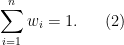
In this post, we study a few probability one results conerning the rank of random matrices: with probability one,
- a random asymmetric matrix has full rank;
- a random symmetric matrix has full rank;
 many random rank one positive semidefinite matrices (belonging to
  ) are linearly independent.
At least for the first two, they look quite natural and should be correct at first glance. However, to rigorously prove them does require some effort. The post is trying to show that one can use the concept of independence to prove the above assertions. Indeed, all the proof follows an inductive argument where independence makes life much easier:
- Draw the first sample, it satisfies the property we want to show,
- Suppose first
 samples satisfy the property we want to show, draw the next sample. Since it is independent of the previous samples, the first samples can be considered as fixed. Then we make some effort to say the first
  sample does satisfy the property.
Before we going into each example, we further note for any probability measure that is absolutely continuous respect to the measure introduced below and vice versa (so independence is not needed), the probability  results listed above still hold.
1. Random Matrices are full rank
Suppose  with
with ![{A=[a_{ij}]}](https://s0.wp.com/latex.php?latex=%7BA%3D%5Ba_%7Bij%7D%5D%7D&bg=ffffff&fg=000000&s=0&c=20201002) and each entry of
and each entry of  is drawn independently from standard Gaussian
  . We prove that
  has rank
  with probability .
To start, we should assume without loss of generality that  . Otherwise, we just repeat the following argument for
  .
.
The trick is to use the independence structure and consider columns of are drawn from left to right. Let’s write the  -th column of by
For the first column, we know  is linearly independent because it is
  with probability . For the second column, because it is drawn independently from the first column, we can consider the first column is fixed, and the probability of
  fall in to the span of a fixed column is because has a continuous density in
  . Thus the first two columns are linearly independent.
For general  , because , we know the first
  columns forms a subspace in and so
  falls into that subspace with probability (linear subspace has Lebesgue measure in and Gaussian measure is absolutely continuous with respect to Lebesgue measure and vice versa). Thus we see first columns are linearly independent. Proceeding the argument until
  completes the proof.
2. Symmetric Matrices are full rank
Suppose  with and each entry of the upper half of ,
  , is drawn independently from standard Gaussian . We prove that has rank
  .
.
Let’s write the -th row of by  . For the first entries of the -th row, we write
  . Similarly,
  denotes the first entries of the -th column. For the top left
  submatrix of , we denote it by
  . Similar notation applies to other submatrices.
The idea is drawing each column of from left to right sequentially and using the independence structure. Starting from the first column, with probability one, we have that is linearly independent (meaning  ).
).
Now since is drawn and the second column except the first entry is independent of , we know it is in the span of if the second column is  (
( is with probability 0) multiple of . This still happens with probability since each entry of
  has continuous probability density and is drawn independently from .
Now assume we have drawn the first columns of , the first columns are linearly independent with probability , and the left top submatrix of is invertible (the base case is what we just proved). We want to show after we draw the column, the first columns are still linearly independent with probability . Since the first columns is drawn, the first entries of the column  is fixed, we wish to show the rest
  entries which are drawn independently from all previous columns will ensure linearly independence of first columns.
Suppose instead is linearly dependent with first columns of . Since the left top submatrix of is invertible, we know there is only one way to write as a linear combination of previous columns. More precisely, we have

This means has to be a fixed vector which happens with probability because the last entries of is drawn independently from ,  Note this implies that the first columns of are linearly independent as well as the left top
  submatrix of is invertible because we can repeat the argument simply by thinking is (instead of
  ). Thus the induction is complete and we prove indeed has rank with probability .
3. Rank positive semidefinite matrices are linearly independent
This time, we consider  ,
,  are drawn independently from standard normal distribution in . Denote the set of symmetric matrices in as
  . We show that with probability the matrices

are linearly independent in .
Denote the standard -th basis vector in as  . First, let us consider the following basis (which can be verified easily) in ,

We order the basis according to the lexicographical order on  . Suppose
  follows standard normal distribution in , we prove that for any fixed linear subspace
  with dimension less than , we have

We start by applying an fixed invertible linear map  to
to  so that the basis of
  is the first
  many basis vector of
  ({in lexicographical order.}), and the basis of the orthogonal complement (defined via the trace inner product) of ,
  , is mapped to the rest of the basis vector of under
  . We then only need to prove

We prove by contradiction. Suppose  . It implies that there exists infinitely many
  such that
  . Moreover, each component of takes infinitely many values. We show such situation cannot occur. Denote the
  -th largest element in
  as
as  . Since has dimension less than ,
  contains nonzero element and so
![\displaystyle \mathcal{F}(\mathbf{a}\mathbf{a}^\top) \in \mathcal{F}(V) \iff [\mathcal{F}(\mathbf{a}\mathbf{a}^\top)]_{ij}=0,\quad \forall (i,j) > (i_0,j_0) \,\text{in lexicographical order.}](https://s0.wp.com/latex.php?latex=%5Cdisplaystyle+%5Cmathcal%7BF%7D%28%5Cmathbf%7Ba%7D%5Cmathbf%7Ba%7D%5E%5Ctop%29+%5Cin+%5Cmathcal%7BF%7D%28V%29+%5Ciff+%5B%5Cmathcal%7BF%7D%28%5Cmathbf%7Ba%7D%5Cmathbf%7Ba%7D%5E%5Ctop%29%5D_%7Bij%7D%3D0%2C%5Cquad+%5Cforall+%28i%2Cj%29+%3E+%28i_0%2Cj_0%29+%5C%2C%5Ctext%7Bin+lexicographical+order.%7D+&bg=ffffff&fg=000000&s=0&c=20201002)
Now fix an  , we know
 ![{ [\mathcal{F}(\mathbf{a}\mathbf{a}^\top)]_{i_1j_1}=0}](https://s0.wp.com/latex.php?latex=%7B+%5B%5Cmathcal%7BF%7D%28%5Cmathbf%7Ba%7D%5Cmathbf%7Ba%7D%5E%5Ctop%29%5D_%7Bi_1j_1%7D%3D0%7D&bg=ffffff&fg=000000&s=0&c=20201002) means that there is some
means that there is some  (depending only on ) such that

where  is the -th complement of . Now if we fix
  and only vary
  , then we have

which holds for infinitely many  only if
Thus we can repeat the argument as before and conclude that  holds for infinitely many with each component taking infinitely many values only if
  . This contradicts the fact that is invertible and hence we must have
Now proving  spans with probability is easy. Because for each , the
  with
with  being drawn can be considered fixed because
  is drawn independently of . But the probability of stays in the span of
  is by previous result and hence is linearly independent of all . This argument continues to hold for
  because the space spanned by
  is at most
  and so previous result applies. This completes the proof.


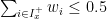


![\displaystyle \partial f(x) = - \sum_{i\in I^-_x} w_i + \sum_{i\in I^+_x} w_i + w_{I_x^=} \times [-1,1], \ \ \ \ \ (4)](https://s0.wp.com/latex.php?latex=%5Cdisplaystyle+%5Cpartial+f%28x%29+%3D+-+%5Csum_%7Bi%5Cin+I%5E-_x%7D+w_i+%2B+%5Csum_%7Bi%5Cin+I%5E%2B_x%7D+w_i+%2B+w_%7BI_x%5E%3D%7D+%5Ctimes+%5B-1%2C1%5D%2C+%5C+%5C+%5C+%5C+%5C+%284%29&bg=ffffff&fg=000000&s=0&c=20201002)
![{w_{I_x^=} \times [-1,1] = [-w_{I_x^=}, w_{I_x^=}]}](https://s0.wp.com/latex.php?latex=%7Bw_%7BI_x%5E%3D%7D+%5Ctimes+%5B-1%2C1%5D+%3D+%5B-w_%7BI_x%5E%3D%7D%2C+w_%7BI_x%5E%3D%7D%5D%7D&bg=ffffff&fg=000000&s=0&c=20201002)
![{w_{I_x^=} \times [-1,1] = 0}](https://s0.wp.com/latex.php?latex=%7Bw_%7BI_x%5E%3D%7D+%5Ctimes+%5B-1%2C1%5D+%3D+0%7D&bg=ffffff&fg=000000&s=0&c=20201002)


![\displaystyle 0 \in \partial f(x) = - \sum_{i\in I^-_x} w_i + \sum_{i\in I^+_x} w_i + w_{I_x^=} \times [-1,1]. \ \ \ \ \ (5)](https://s0.wp.com/latex.php?latex=%5Cdisplaystyle+0+%5Cin+%5Cpartial+f%28x%29+%3D+-+%5Csum_%7Bi%5Cin+I%5E-_x%7D+w_i+%2B+%5Csum_%7Bi%5Cin+I%5E%2B_x%7D+w_i+%2B+w_%7BI_x%5E%3D%7D+%5Ctimes+%5B-1%2C1%5D.+%5C+%5C+%5C+%5C+%5C+%285%29&bg=ffffff&fg=000000&s=0&c=20201002)


 and
and  . The dual program is accordingly
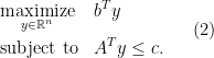
 that are feasible for
 , hence the above condition is equivalent to
 , and using the feasibility
  and
and  , we conclude
 ![\displaystyle \textbf{complementarity:} \quad x_i [z(y) ]_i= 0 \quad \text{for all}\;1\leq i\leq n. \ \ \ \ \ (5)](https://s0.wp.com/latex.php?latex=%5Cdisplaystyle++%5Ctextbf%7Bcomplementarity%3A%7D+%5Cquad+x_i+%5Bz%28y%29+%5D_i%3D+0+%5Cquad+%5Ctext%7Bfor+all%7D%5C%3B1%5Cleq+i%5Cleq+n.+%5C+%5C+%5C+%5C+%5C+%285%29&bg=ffffff&fg=000000&s=0&c=20201002)
 and
and ![{[z(y)]_i}](https://s0.wp.com/latex.php?latex=%7B%5Bz%28y%29%5D_i%7D&bg=ffffff&fg=000000&s=0&c=20201002) are
are  respectively. The above derivation shows that strong duality
  .
.![\displaystyle \textbf{strict complementarity:} \quad \text{for all}\; i \quad x_i = 0 \iff [z(y^*)]_i > 0. \ \ \ \ \ (6)](https://s0.wp.com/latex.php?latex=%5Cdisplaystyle++%09%5Ctextbf%7Bstrict+complementarity%3A%7D+%5Cquad+%5Ctext%7Bfor+all%7D%5C%3B+i+%5Cquad+x_i+%3D+0+%5Ciff+%09%5Bz%28y%5E%2A%29%5D_i+%3E+0.+%5C+%5C+%5C+%5C+%5C+%286%29&bg=ffffff&fg=000000&s=0&c=20201002)
 , there either exists a primal optimal
  or there exists a dual optimal
  such that
 ![{[z(y)]_j >0}](https://s0.wp.com/latex.php?latex=%7B%5Bz%28y%29%5D_j+%3E0%7D&bg=ffffff&fg=444444&s=0&c=20201002) .
.  , either there is an optimal
  such that
  or there is an optimal
  such that
 ![{[z(y^j)]_j >0}](https://s0.wp.com/latex.php?latex=%7B%5Bz%28y%5Ej%29%5D_j+%3E0%7D&bg=ffffff&fg=000000&s=0&c=20201002) but not both due to
but not both due to  be the subset of
  consists of
  such that
  . Consequently, using Lemma
  consists of indices s.t. an optimal
 ![{[z(y^j)]_j>0}](https://s0.wp.com/latex.php?latex=%7B%5Bz%28y%5Ej%29%5D_j%3E0%7D&bg=ffffff&fg=000000&s=0&c=20201002) . Then the desired
. Then the desired 
 is the cardinality of
  . Fix an index
 is the
 such that
 , then
  is optimal for
 ![\displaystyle c - A^\top\left( \frac{y}{\lambda} \right)\geq \frac{1}{\lambda }e_j \implies [z(\frac{y}{\lambda})]_j >0. \ \ \ \ \ (11)](https://s0.wp.com/latex.php?latex=%5Cdisplaystyle++%09c+-+A%5E%5Ctop%5Cleft%28+%5Cfrac%7By%7D%7B%5Clambda%7D+%5Cright%29%5Cgeq+%5Cfrac%7B1%7D%7B%5Clambda+%7De_j+%5Cimplies+%5Bz%28%5Cfrac%7By%7D%7B%5Clambda%7D%29%5D_j+%3E0.+%5C+%5C+%5C+%5C+%5C+%2811%29&bg=ffffff&fg=000000&s=0&c=20201002)
 . Then
  and
and  . Now take any
  that is optimal for
  satisfies the conclusion in Lemma
 ![{[z(y)]_j>0}](https://s0.wp.com/latex.php?latex=%7B%5Bz%28y%29%5D_j%3E0%7D&bg=ffffff&fg=000000&s=0&c=20201002) . Suppose we are now in the second situation. Then this directly means that there is a feasible
. Suppose we are now in the second situation. Then this directly means that there is a feasible  .
. on real line
  where
where  and
and  means “independently and identically distributed as”. We denote
  to be the
  -th largest random variable of the
  s. So
s. So  is the largest value and
  is the smallest of the
  s. Note here the subscript
  does not mean taking to the
  are called order statistics in Statistics. They are
  ,
,  and
and 

 -th largest value. The left inequalities of the inequality
  -th order statistic is in expectation.
 and take
  ,
,  , and
, and  in Theorem
 , then we can take
  ,
,  . Then equation

 and
and 
 and
and  are interlacing. The main idea of the proof is putting
  and
and  and
and  in the same probability space and arguing that we actually have almost sure inequality instead of just expectation or stochastically dominance. This technique is known as coupling.
  many more
  follows
  . We now consider all the

 -th largest value
  is always smaller than the

 have joint distribution
  . Denote
  to be the order statistics. Now consider only the first
  . Denote their marginal distribution as
  . We denote the order statistics of these
  . Then for any
  and
and 

 and order them so that we have
  s. Now if we generate the extra
  and the first
 is at most
  since we have

 s, the
  is always smaller than the

 for any
  .
.  with parameter (index)
  is said to be a natural exponential family if
 , we call
 : natural sufficient statistic
 : natural parameter
 : natural parameter space.
 ,
,  , and a random variable
  , a statistic
 is independent of
  . A sufficient statistic
  , there is a function
  such that
  .
. according to
  ! So even though you don’t know the underlying distribution
  is
is .
.
 .
.
 for the integral
  to be finite and
  for the integral
  to be finite. This means actually
  and so the natural parameter space is a single point
  .
. is indeed sufficient. But any constant estimator is also sufficient and minimal as any other sufficient statistic under a constant function is a constant. But
  , if
, if  , i.e.,
  is nonnegative as well, is there any relation with their singular values?
 , is larger than the largest singular value of
  ,
,  :
:
 are symmetric, so that
  ,
,  . Here for any symmetric matrix
  , we denote its eigenvalues as
  .
. are all nonnegative and symmetric, then
 corresponding to the eigenvalue
  , which is both nonnegative and largest in magnitude. Next, by multiplying left and right of
  and
and 
 is because
  is because
  . The step
  is because
  . The step
  is because
  are symmetric and both are nonnegative so largest eigenvalue is indeed just the singular value due to Perron-Frobenius theorem.
  are all nonnegative, then
 and
and  in
in  :
:
 , we also have
  . Using Lemma
  in this case by considering
 , how do you test that
  s all come from the same distribution, i.e., how do you test homogeneity of the data?
 , i.e., a set
 for some
  ?
? (known as the identifiability of
  ?
? has a density
  is
is


 and the space of the alternative as
  . A popular and natural approach is the likelihood ratio test. We construct the test statistic which is called likelihood ratio as
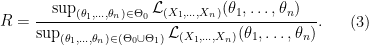
 such that
  and
and  , then this ratio should be large and we have confidence that our null hypothesis is true. This means we should reject our null hypothesis if we find
  is small. Thus if we want to have a significance level
  test of our null hypothesis, we should reject null hypothesis when
  where
where  satisfies
 even if we know how to sample from each
 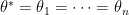 ) generates the data. So the distribution of
 through computational methods, we have to simulate for each
  . As
. As  could be rather large (in fact as large as
  ), approximation can be time consuming as well.
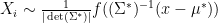
 is the so called location-scale family, we find that the distribution of
  indexed by
  where
where  and
and  , the set of invertible matrices in
  . The family
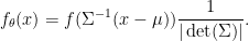
 follows
  has probability density
  . Indeed, for any Borel set
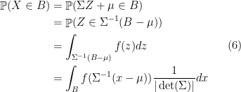
 in the last equality and the last equality shows
  such that each
  and the distribution of
  , and any
 and
and  where
where 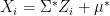 . Then the likelihood of
  is
is 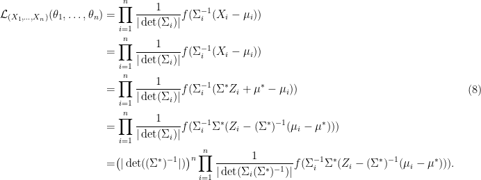

 ,
,  ,
,  and
and 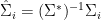 . Note that since
  ,
,  can vary all over the space
  , so is
  ,
,  and
and  . The equality
 and
and  at all. So our theorem is proved.
  , a convex function
  where
where  is a convex set and an
  , if
, if  or
or  , then
![\displaystyle \begin{aligned} \partial (\phi \circ h) (x) = \phi' (h(x)) \cdot[ \partial h (x)], \end{aligned} \ \ \ \ \ (1)](https://s0.wp.com/latex.php?latex=%5Cdisplaystyle+%5Cbegin%7Baligned%7D+%5Cpartial+%28%5Cphi+%5Ccirc+h%29+%28x%29+%3D+%5Cphi%27+%28h%28x%29%29+%5Ccdot%5B+%5Cpartial+h+%28x%29%5D%2C+%5Cend%7Baligned%7D+%5C+%5C+%5C+%5C+%5C+%281%29&bg=ffffff&fg=000000&s=0&c=20201002)
 is the operator of taking subdifferentials of a function, i.e.,
  for any
  is the interior of
  with respect to the standard topology in
  for all
  defined on
 ![{[0,1]}](https://s0.wp.com/latex.php?latex=%7B%5B0%2C1%5D%7D&bg=ffffff&fg=000000&s=0&c=20201002) . Then
. Then ![{[0,1],\phi'(0) = 0}](https://s0.wp.com/latex.php?latex=%7B%5B0%2C1%5D%2C%5Cphi%27%280%29+%3D+0%7D&bg=ffffff&fg=000000&s=0&c=20201002) ,
, ![{\partial h(0) =(-\infty,0]}](https://s0.wp.com/latex.php?latex=%7B%5Cpartial+h%280%29+%3D%28-%5Cinfty%2C0%5D%7D&bg=ffffff&fg=000000&s=0&c=20201002) . However, in this case
. However, in this case ![{\partial (\phi\circ h)(0)= (-\infty,0]}](https://s0.wp.com/latex.php?latex=%7B%5Cpartial+%28%5Cphi%5Ccirc+h%29%280%29%3D+%28-%5Cinfty%2C0%5D%7D&bg=ffffff&fg=000000&s=0&c=20201002) and
and ![{\phi' (h(0)) \cdot[ \partial h (0)] =0}](https://s0.wp.com/latex.php?latex=%7B%5Cphi%27+%28h%280%29%29+%5Ccdot%5B+%5Cpartial+h+%280%29%5D+%3D0%7D&bg=ffffff&fg=000000&s=0&c=20201002) . Thus, the equality fails.
. Thus, the equality fails. is also differentiable, then the above reduces to the common chain rule of smooth functions.
![{\partial (\phi \circ h) (x) \supset \phi' (h(x)) \cdot[ \partial h (x)]}](https://s0.wp.com/latex.php?latex=%7B%5Cpartial+%28%5Cphi+%5Ccirc+h%29+%28x%29+%5Csupset+%5Cphi%27+%28h%28x%29%29+%5Ccdot%5B+%5Cpartial+h+%28x%29%5D%7D&bg=ffffff&fg=000000&s=0&c=20201002) . We have for all
. We have for all  ,
,
 are just the definition of subdifferential of
  at
at  and
and  in the inequality
  such that
  is not empty. Let
  , we wish to show that
 ![{ \phi' (h(0)) \cdot[ \partial h (0)]}](https://s0.wp.com/latex.php?latex=%7B+%5Cphi%27+%28h%280%29%29+%5Ccdot%5B+%5Cpartial+h+%280%29%5D%7D&bg=ffffff&fg=000000&s=0&c=20201002) . First according to the definition of subdifferential, we have
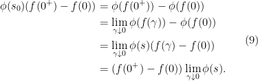
. First according to the definition of subdifferential, we have
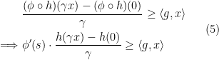
![\displaystyle \begin{aligned} (\phi \circ h) (\gamma x)\geq (\phi\circ h)(0) + \langle{ g} ,{\gamma x}\rangle, \forall x \in U, \gamma \in [0,1]. \end{aligned} \ \ \ \ \ (4)](https://s0.wp.com/latex.php?latex=%5Cdisplaystyle+%5Cbegin%7Baligned%7D+%28%5Cphi+%5Ccirc+h%29+%28%5Cgamma+x%29%5Cgeq+%28%5Cphi%5Ccirc+h%29%280%29+%2B+%5Clangle%7B+g%7D+%2C%7B%5Cgamma+x%7D%5Crangle%2C+%5Cforall+x+%5Cin+U%2C+%5Cgamma+%5Cin+%5B0%2C1%5D.+%5Cend%7Baligned%7D+%5C+%5C+%5C+%5C+%5C+%284%29&bg=ffffff&fg=000000&s=0&c=20201002)
 between
  and
and  by mean value theorem. Now, by letting
  , if
, if  is nondecreasing in
 , then dividing both sides of the above inequality by
  gives
gives 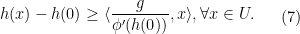
 is indeed a member of
  and thus
 ![{\partial (\phi \circ h) (x) \subset \phi' (h(x)) \cdot[ \partial h (x)]}](https://s0.wp.com/latex.php?latex=%7B%5Cpartial+%28%5Cphi+%5Ccirc+h%29+%28x%29+%5Csubset+%5Cphi%27+%28h%28x%29%29+%5Ccdot%5B+%5Cpartial+h+%28x%29%5D%7D&bg=ffffff&fg=000000&s=0&c=20201002) . In this case, we only need to verify why
. In this case, we only need to verify why  must be right continuous at
  , then
  , using the inequality
 , then
  and it indeed belongs to the set
 ![{\phi' (h(0)) \cdot[ \partial h (x)] = \{0\}}](https://s0.wp.com/latex.php?latex=%7B%5Cphi%27+%28h%280%29%29+%5Ccdot%5B+%5Cpartial+h+%28x%29%5D+%3D+%5C%7B0%5C%7D%7D&bg=ffffff&fg=000000&s=0&c=20201002) as
as  for
for  is indeed right continuous at
  exists and
  . Now if
  , then
  . But in this case
  is going to be negative infinity as
  . Recall from inequality
 ,
,  approaches a positive number. If this claim is true, then from the above inequality, we will have
 . Using mean value theorem, we have for some
 ![{s_0 \in [ f(0^+), f(0)]}](https://s0.wp.com/latex.php?latex=%7Bs_0+%5Cin+%5B+f%280%5E%2B%29%2C+f%280%29%5D%7D&bg=ffffff&fg=000000&s=0&c=20201002)
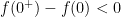 above, we see that
  . We claim
  . If
. If  , then because
 ![{[f(0^+),f(0)]}](https://s0.wp.com/latex.php?latex=%7B%5Bf%280%5E%2B%29%2Cf%280%29%5D%7D&bg=ffffff&fg=000000&s=0&c=20201002) as
as  . This contradicts our assumption that
  and our proof is complete.
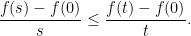
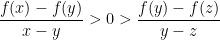
 ![{f:[0,1]\rightarrow \mathbb{R}}](https://s0.wp.com/latex.php?latex=%7Bf%3A%5B0%2C1%5D%5Crightarrow+%5Cmathbb%7BR%7D%7D&bg=ffffff&fg=000000&s=0&c=20201002) be a (strictly) convex function, then the function
be a (strictly) convex function, then the function ![{g(x) = \frac{f(x)-f(0)}{x}, x\in(0,1]}](https://s0.wp.com/latex.php?latex=%7Bg%28x%29+%3D+%5Cfrac%7Bf%28x%29-f%280%29%7D%7Bx%7D%2C+x%5Cin%280%2C1%5D%7D&bg=ffffff&fg=000000&s=0&c=20201002) is non-decreasing (strictly increasing).
is non-decreasing (strictly increasing). 
 by
by  .
.  where
where  is any connected set in
  , we have
 where
where ![{[a,b],(a,b),(a,b],[a,b)}](https://s0.wp.com/latex.php?latex=%7B%5Ba%2Cb%5D%2C%28a%2Cb%29%2C%28a%2Cb%5D%2C%5Ba%2Cb%29%7D&bg=ffffff&fg=000000&s=0&c=20201002) where
where  . Then
  all in

 are interior point of
 ![{[x,z]}](https://s0.wp.com/latex.php?latex=%7B%5Bx%2Cz%5D%7D&bg=ffffff&fg=000000&s=0&c=20201002) . This means that
. This means that  as
as  . Now for any
  , by convexity and monotonicity of slope, we have
 . Thus
 ![{I\cap (-\infty,x_0]}](https://s0.wp.com/latex.php?latex=%7BI%5Ccap+%28-%5Cinfty%2Cx_0%5D%7D&bg=ffffff&fg=000000&s=0&c=20201002) . Similarly, using monotonicity of slope, we have
. Similarly, using monotonicity of slope, we have  . Now if suppose either
  is the end point of
  . Then there are only three possible cases


 are interior point and we can proceed our previous argument and show
  and ask the relation between
  and
and  . The only non-ideal case is that
  (the other case gives three interior point such that
  and we can employ our previous argument). We can then further have
  . Again there will be only one non-ideal case that
  .
. or the sequence
  satisfies
  for all
  . If
. If  . But this is not possible because
  . Thus
  . Indeed, for any
  for
for  , there is a
  and so
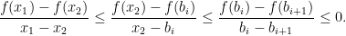
 , we see
 ![{f:[a,b] \rightarrow \mathbb{R}}](https://s0.wp.com/latex.php?latex=%7Bf%3A%5Ba%2Cb%5D+%5Crightarrow+%5Cmathbb%7BR%7D%7D&bg=ffffff&fg=000000&s=0&c=20201002) is convex for some
is convex for some  . Then
  .
.  on
on  and the point
  .
.
 . The dual of the standard form is
 to Program
 be the optimal value of Program
  be an optimal solution to the same program. We would like to ask the following question:
 , only induces small changes in the optimal value and solution. The reason is that in real application, there might be some error in the coding of
  or even
 be
be  and the set of extreme rays be
  . Using our assumption A1, we know


 is bounded, then we have
  where
where  has all column independent. Here
  is the submatrix of
  . By complementarity of LP
 . What we have done is that under A1 and A2,
 .
.


 is the dual norm of
  . We note
  here is arbitrary.
 and
and  are arbitrary norms. We conclude the above discussion in the following theorem.
 is the set of extreme points of the feasible region of
  is the set of extreme points of the feasible region of
  . Under assumption A1 and A2, we have for all
  ,
,
 are arbitrary norms. Here
  .
.
