LP Conditioning

We consider global conditioning property of Linear Program (LP) here. Let’s first define the problem. The standard form of LP is

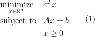
$\displaystyle \begin{aligned} & \underset{x \in \mathbb{R}^n}{\text{minimize}} & & c^Tx\\ & {\text{subject to}} & & Ax =b ,\\ & & & x\geq 0 \end{aligned} \ \ \ \ \ (1)$

where ${A \in \mathbb{R}^{n\times m}, c\in \mathbb{R}^n}$ and ${b \in\mathbb{R}^m}$ . The dual of the standard form is

$\displaystyle \begin{aligned} & \underset{y \in \mathbb{R}^m}{\text{maximize}} & & b^Ty\\ & {\text{subject to}} & & A^Ty\leq c. \\ \end{aligned} \ \ \ \ \ (2)$

Now suppose we add perturbation ${u\in \mathbb{R}^{n}}$ to Program (2) in the ${c}$ term, we have

$\displaystyle \begin{aligned} & \underset{y \in \mathbb{R}^n}{\text{maximize}} & & b^Ty\\ & {\text{subject to}} & & A^Ty\leq c+u.\\ \end{aligned} \ \ \ \ \ (3)$

Let ${v(u)}$ be the optimal value of Program (3) and ${y(u)}$ be an optimal solution to the same program. We would like to ask the following question:

$\displaystyle \begin{aligned} \textbf{Q}&: \text{Is}\; v(u)\; \text{Lipschitz continuous?} \;\text{Is} \;y(u)\;\text{Lipschitz}? \end{aligned} \ \ \ \ \ (4)$

Such questions are called the conditioning of Program (2). It asks under some perturbation, how does the solution and optimal value changes accordingly. In general, we hope that Program (1) and (2) to be stable in the sense that small perturbation in the data, i.e., ${A,b,c}$ , only induces small changes in the optimal value and solution. The reason is that in real application, there might be some error in the coding of ${b,c}$ or even ${A}$ . If Program (1) and (2) are not stable with respect to the perturbation, then possibly either more costs need to be paid to the encoding of the data or the LP is not worth solving. At first sight, it is actually not even clear that

Whether ${v(u)}$ will be always finite?
Whether ${y(u)}$ is actually unique? If ${y(u)}$ is not unique, then the Lipschitz property of ${y(u)}$ does not even make sense.

To address the first issue, we make our first assumption that

A1: Program (2) has a solution and the optimal value is finite.

Under A1, by strong duality of LP, we have that Program (1) also has a solution and the optimal value is the same as the optimal value of Program (2). This, in particular, implies that (1) is feasible. We now characterize the region where ${v(u)}$ is finite. Let the feasible region of Program (1) be denoted as

$\displaystyle \mathcal{F}_p :\,= \{x\mid Ax = b,x\geq 0\},$

the set of vertices of ${\mathcal{F}_p}$ be ${\mathcal{V}_p=\{x_i\}_{i=1}^d}$ and the set of extreme rays be ${\mathcal{R}_p=\{\gamma_j\}_{j=1}^l}$ . Using our assumption A1, we know

$\displaystyle \mathcal{F}_p \not = \emptyset.$

Now according to the Resolution Theorem of the primal polyhedron, we have

$\displaystyle \mathcal{F}_p = \{ x\mid x = \sum_{i=1}^d \alpha _ix_i + \sum_{j=1}^l\beta_j \gamma_j, x_i \in \mathcal{V}_p, \gamma _j \in \mathcal{R}_p,\sum_{i=1}^d \alpha_i =1, \alpha_i\geq 0, \beta_j \geq 0, \forall i,j\}.$

Using this representation, the fact that the primal of Program (3) is

$\displaystyle \begin{aligned} & \underset{x \in \mathbb{R}^n}{\text{minimize}} & & (c+u)^Tx\\ & {\text{subject to}} & & Ax =b \\ & & & x\geq 0, \end{aligned} \ \ \ \ \ (5)$

and strong duality continue to hold for (3) and (5) as (5) is feasible by A1, the value of ${v(u)}$ is

$\displaystyle v(u) = \min \{ c^Tx_i +u^Tx_i\mid x_ i \in \mathcal{V}_p\} + \min\{c^T\gamma_j +\beta_ju^T\gamma_j \mid \gamma_j \in \mathcal{R}_p,\beta_j\geq 0\}.$

Thus it is immediate that the region where ${v(u)}$ is finite is

$\displaystyle \begin{aligned} \mathcal{F}_u = \{ u\mid \gamma_j ^Tu\geq 0, \forall \gamma_j \in \mathcal{R}_p\}. \end{aligned} \ \ \ \ \ (6)$

In particular, if ${\mathcal{F}_p}$ is bounded, then we have ${v(u)}$ to be always finite.

To address the issue whether ${y(u)}$ is unique, we make the following nondegenerate assumption on vertices.

A2: All the basic feasible solution of (1) are non-degenerate, i.e., all vertices of the feasible region of Program (1) have exactly ${m}$ positive entries.

Under this condition, and the definition of basic feasible solution, we know if ${x}$ is a basic feasible solution, then ${A_{\cdot V(x)}\in \mathbb{R}^{m\times m}}$ where ${V(x)=\{i\mid x_i \text{ is nonzero}\}}$ has all column independent. Here ${A_{\cdot V(x)}}$ is the submatrix of ${A}$ having columns with indices in ${\mathcal{V}(x)}$ . By complementarity of LP (3) and (5), we thus know that if ${x}$ is a baisc feasible solution and it is a solution to Program (5), then

$\displaystyle y(u) = (A_{\cdot V(x)})^{-T}(c+u)$

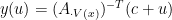
is the unique solution to Program (3) where ${(A_{\cdot V(x)})^{-T} =((A_{\cdot V(x)})^{T})^{-1} }$ . What we have done is that under A1 and A2,

$\displaystyle v(u) = \min \{ c^Tx_i +u^Tx_i, x_ i \in \mathcal{V}_p\}, u \in \mathcal{F}_u$

and

$\displaystyle y(u) = (A_{\cdot V(x)})^{-T}(c+u)$

where ${x = \arg\min_{x_i}\{ c^Tx_i +u^Tx_i, x_ i \in \mathcal{V}_p\}}$ .

By defining

$\displaystyle \Omega_i = \{ u \mid c^Tx_i +u^Tx_i \leq c^Tx_j +u^Tx_j,\forall j\not =i \}, \forall\, 1\leq i\leq d$

which is a polyhedron, we may write the above compactly as

$\displaystyle v(u) = c^Tx_i +u^Tx_i, \quad y(u) = (A_{\cdot V(x_i)})^{-T}(c+u), u \in \Omega_i.$

Then it is easy to see that the Lipschitz condition of ${v(u)}$ is

$\displaystyle |v(u_1)-v(u_2)| \leq \max\{\|x_i\|_*,x_i \in \mathcal{V}_p\|\} \|u_1-u_2\|$

where ${\|\cdot\|_*}$ is the dual norm of ${\|\cdot\|}$ . We note ${\|\cdot \|}$ here is arbitrary.

Similarly, by using the theorem in this post, we see that ${y(u)}$ is also Lipschitz continuous with Lipschitz property

$\displaystyle \| y(u_1) - y(u_2)\|_\alpha \leq\max \{ \|(A_{\cdot V(x)})^{-T}\|_{\alpha,\beta }, x \in \mathcal{V}_p\}\|u_1-u_2\|_{\beta }$

where ${\|(A_{\cdot V(x)})^{-T}\|_{\alpha,\beta } = \max_{\|x\|_{\beta }=1}\|(A_{\cdot V(x)})^{-T}\|_\alpha}$ and ${\|\cdot\|_\alpha, \|\cdot\|_\beta}$ are arbitrary norms. We conclude the above discussion in the following theorem.

Theorem 1 Recall ${\mathcal{V}_p}$ is the set of extreme points of the feasible region of (1), ${\mathcal{R}_p}$ is the set of extreme points of the feasible region of (1) and ${\mathcal{F}_u = \{ u\mid \gamma_j ^Tu\geq 0, \forall \gamma_j \in \mathcal{R}_p\}}$ . Under assumption A1 and A2, we have for all ${x\in \mathcal{F}_u}$ ,

$\displaystyle |v(u_1)-v(u_2)| \leq \max\{\|x_i\|_*,x_i \in \mathcal{V}_p\|\} \|u_1-u_2\|$

and

$\displaystyle \| y(u_1) - y(u_2)\|_\alpha \leq\max \{ \|(A_{\cdot V(x)})^{-T}\|_{\alpha,\beta }, x \in \mathcal{V}_p\}\|u_1-u_2\|_\beta$

where ${\|\cdot\|,\|\cdot\|_{\alpha},\|\cdot\|_\beta }$ are arbitrary norms. Here ${A_{\cdot V(x)}}$ is the submatrix of ${A}$ having columns with indices in ${\mathcal{V}(x)=\{i\mid x_i \text{ is nonzero}\}}$ .

How might one bound the Lipschitz constants

$\displaystyle \max\{\|x_i\|_*,x_i \in \mathcal{V}_p\|\} \text{ and } \max \{ \|(A_{\cdot V(x)})^{-T}\|_{\alpha,\beta }, x \in \mathcal{V}_p\}?$

The former might be done by giving a bound of the diameter of the feasible region ${\mathcal{F}_p}$ of Program (1) and the later might be done through some restricted isometry property of ${A}$ .

One thought on “LP Conditioning”

Beiyi

March 16, 2018 at 2:40 am

立君你好棒呀😊

LikeLiked by 1 person

Three Squirrels

Little Discoveries of Optimization, Statistics, and Probability

LP Conditioning

One thought on “LP Conditioning”

Leave a Reply Cancel reply

Share this:

Like this:

Related

One thought on “LP Conditioning”

Leave a Reply Cancel reply