Suppose you have a sequence of independent data 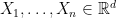 , how do you test that
  s all come from the same distribution, i.e., how do you test homogeneity of the data?
To make the problem more precise, suppose we have a distribution family indexed by  , i.e., a set

and each follows the distribution  for some
  . Our problem is
Is  ?
?
If we have that  (known as the identifiability of
  ), then our question becomes
Is  ?
?
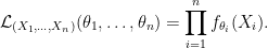
Now suppose further that each  has a density
  (so that we can write down the likelihood), the likelihood of seeing the independent sequence
  is
is
To test our question in a statistical way, we use hypothesis testing. Our null hypothesis is

and our alternative hypothesis is

Further denote the space of the null as  and the space of the alternative as
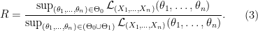
  . A popular and natural approach is the likelihood ratio test. We construct the test statistic which is called likelihood ratio as
Intuitively, if our null hypothesis is indeed true, i.e., there is some  such that
  and follows
  , then this ratio should be large and we have confidence that our null hypothesis is true. This means we should reject our null hypothesis if we find
  is small. Thus if we want to have a significance level
  test of our null hypothesis, we should reject null hypothesis when
  where
where  satisfies

However, the main issue is that we don’t know the distribution of under  even if we know how to sample from each and the functional form of for each . The reason is that did not specify which (which equals to
  ) generates the data. So the distribution of may depend on as well and the real thing we need for is

Thus even if we want to know approximate the  through computational methods, we have to simulate for each
  . As
. As  could be rather large (in fact as large as
  ), approximation can be time consuming as well.
Fortunately, if  is the so called location-scale family, we find that the distribution of is independent of and we are free to chose whichever we like. Let us define what is location-scale family, then state the theorem and prove it.
Definition 1 Suppose we have a family of probability densities on  indexed by
  where
where  and
and  , the set of invertible matrices in
  . The family is a local-scale family if there is a family member
  (called pivot) such that for any other with ,
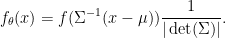
Thus if  follows , then
  has probability density
  . Indeed, for any Borel set
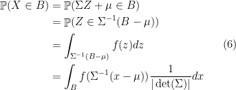
where we use a change of variable  in the last equality and the last equality shows
  follows . We are now ready to state the theorem and prove it.
Theorem 2 Suppose our family of distribution is a local-scale family, then under the null hypothesis, there is a  such that each follows
  and the distribution of is independent of .
Since the distribution of is independent of under the null. This means that for any  , and any

Thus we can choose any family member of to sample and approximates the distribution of using empirical distribution as long as is a location-scale family!
Proof: We need to show that the ratio has distribution independent of . Since 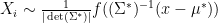 and is a location scale family, we can assume they are generated via
  where follows a pivot and
 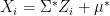 . Then the likelihood of
  is
is
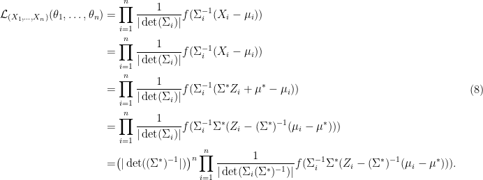
Thus the likelihood ratio reduces to

Now let’s define  ,
,  ,
,  and
and 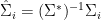 . Note that since
  ,
,  can vary all over the space
  , so is
  ,
,  and
and  . The equality (10) can be rewritten as

As we just argued, , and can vary all over the space without any restriction, the supremum in the numerator and denominator thus does not depend on the choice  and
and  at all. So our theorem is proved.

There is a small typo in Theorem 2. In the density function of X_i, it should be (x – \mu^*) instead of (x – \mu).
LikeLiked by 1 person
Thanks! I fixed it.
LikeLike
The likelihood ratio will converge in distribution to a chi-square distribution. If X does not follow a location-scale distribution, is this asymptotic results still true? Will the chi-square approximation perform well in a finite sample?
LikeLike
I think the asymptotic result that likelihood ratio converging to a chi-square distribution is not specific to location-scale family. For finite sample, I don’t know whether chi-square approximation is good or bad.
LikeLike