June | 2023 | Three Squirrels

We consider the following ${\ell_1}$ minimization problem:

$\displaystyle \begin{aligned} & \underset{x \in \mathbb{R} }{\text{minimize}} & &f(x):\,= \sum_{i=1}^n w_i | x - b_i|. \end{aligned} \ \ \ \ \ (1)$

The weights ${w_i}$ are all positive and ${b_i \in \mathbb{R}}$ . We call the optimziation problem (1) the least absolute deviation problem. Note the optimziation problem (1) has a single variable ${x}$ . If ${w_i}$ are all equal, then it is well-known that least absolute deviation has median of ${\{b_i\}_{i=1}^n}$ as its minimizer. In the case of unequal weights ${w_i}$ , we are going to show the median defined by the weights ${w_i}$ is again the minimizer.

To make the presentation simpler, we assume the weights are normalized:

$\displaystyle \sum_{i=1}^n w_i = 1. \ \ \ \ \ (2)$

Without loss of generality, we assume the values ${b_i}$ are ordered and distinct:

$\displaystyle b_1 <b_2<\dots < b_n. \ \ \ \ \ (3)$

Next, we give the definition of median of ${\{b_i\}_{i=1}^n}$ with respect to the weights ${\{w_i\}_{i=1}^n}$ . For each ${x\in \mathbb{R}}$ , we denote ${I_x^-}$ , ${I_x^=}$ , and ${I_x^+}$ be the set of indices ${i}$ such that ${x<b_i}$ , ${x=b_i}$ , and ${x>b_i}$ respectively. Note that ${I_x^=}$ is either a single index or an empty set.

Definition 1 We say an ${x}$ is a median of ${\{b_i\}_{i=1}^n}$ with respect to the weights ${\{w_i\}_{i=1}^n}$ if ${\sum_{i\in I^+_x} w_i \leq 0.5}$ and ${\sum_{i\in I^+_x} w_i + w_{I^=_x} \geq 0.5}$ , where ${w_{I^=_x} =0}$ if ${I^=_x}$ is empty.

Note that under this definition, the median is acutally not always unique.

We now state the theorem that asserts the optimal solution to (1) is the weighted median.

Theorem 2 Under assumption (2) and (3), the optimal solution to (1) is any median ${x}$ in the sense of Definition 1.

The key of the proof is to note that (1) is convex and a point ${x}$ is optimal if and only if ${ 0 \in \partial f(x)}$ , where ${\partial f(x)}$ is the subdifferential of ${f}$ at ${x}$ , a generalization of derivative at ${x}$ .

Proof: For any ${x\in \mathbb{R}}$ , the subdifferential at ${x}$ is

$\displaystyle \partial f(x) = - \sum_{i\in I^-_x} w_i + \sum_{i\in I^+_x} w_i + w_{I_x^=} \times [-1,1], \ \ \ \ \ (4)$

where ${w_{I_x^=} \times [-1,1] = [-w_{I_x^=}, w_{I_x^=}]}$ if ${I_x^=}$ is nonempty and ${w_{I_x^=} \times [-1,1] = 0}$ if ${I_x^=}$ is empty. The addition in (4) should be understood as set addition: ${A+B = \{a+b \mid a\in A, b\in B\}}$ .

Since the function ${f}$ is a convex function with whole domain ${\mathbb{R}}$ . Hence, an ${x}$ is optimal if and only if

$\displaystyle 0 \in \partial f(x) = - \sum_{i\in I^-_x} w_i + \sum_{i\in I^+_x} w_i + w_{I_x^=} \times [-1,1]. \ \ \ \ \ (5)$

From the the definition of median and the assumption that the weights added up to 1, it is immediate that the median satisfies the above condition and any solution satisfies the above condition is a median. $\Box$

From the Theorem 2, we know that we only need to compute the median of ${\{b_i\}_{i=1}^n}$ w.r.t. ${\{w_i\}_{i=1}^n}$ . This can be computed first by ordering the ${b_i}$ so that condition (3) is satisfied (combining same quantities). This procedure only takes ${\mathcal{O}(n\log n)}$ comparisons plus ${\mathcal{O}(n)}$ operations in creating a new set of values ${\{b'_i\}_{i=1}^{n'}}$ and their weights ${\{w_i'\}_{i=1}^{n'}}$ of combining terms and adding weights up for the same ${b_i}$ . Here ${n'\leq n}$ . Then we add ${w_i'}$ up until the ${0.5}$ threshold is reached to determine ${i}$ . This procedure again only takes ${\mathcal{O}(n)}$ additions.

This note will show the following:

strict complementarity always holds for feasible linear programs (LPs).

This result is known in a very early paper by Goldman and Tucker (1956). Here we aim to give a constructive and hopefully easy to understand proof.

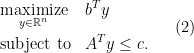
To explain the meaning of this statement, let us start with the the standard form of LP as the primal program

$\displaystyle \begin{aligned} & \underset{x \in \mathbb{R}^n}{\text{minimize}} & & c^Tx\\ & {\text{subject to}} & & Ax =b ,\\ & & & x\geq 0 \end{aligned} \ \ \ \ \ (1)$

where ${A \in \mathbb{R}^{n\times m}, c\in \mathbb{R}^n}$ and ${b \in\mathbb{R}^n}$ . The dual program is accordingly

$\displaystyle \begin{aligned} & \underset{y \in \mathbb{R}^n}{\text{maximize}} & & b^Ty\\ & {\text{subject to}} & & A^Ty\leq c. \\ \end{aligned} \ \ \ \ \ (2)$

Let us now introduce the concept strict complementarity. We start with complementarity, which is a consequence of strong duality. Indeed, suppose that primal (1) and (2) are both feasible. Hence according to LP strong duality, we know there is a primal and dual pair ${(x,y)\in \mathbb{R}^n \times \mathbb{R}^n}$ that are feasible for (1) and (2) respectively, and

$\displaystyle \textbf{strong duality:}\quad c^\top x = b^\top y. \ \ \ \ \ (3)$

Using the fact ${x}$ is feasible, we know ${Ax = b}$ , hence the above condition is equivalent to

$\displaystyle 0 = c^\top x - (Ax) ^\top y =(c- A^\top y)^\top x. \ \ \ \ \ (4)$

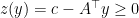Letting the slack map ${z (y) = c-A^\top y}$ , and using the feasibility ${x\geq 0 }$ and ${z(y) = c - A^\top y\geq 0}$ , we conclude

$\displaystyle \textbf{complementarity:} \quad x_i [z(y) ]_i= 0 \quad \text{for all}\;1\leq i\leq n. \ \ \ \ \ (5)$

Here ${x_i}$ and ${[z(y)]_i}$ are ${i}$ -th element of ${x}$ and ${z(y)}$ respectively. The above derivation shows that strong duality (3) and complementarity (5) are equivalent for feasible ${x}$ and ${y}$ .

The equality (5) implies that at least one of ${x_i}$ and ${[z(y)]_i}$ has to be ${0}$ . However, it is possible that both term are zero. Strict complementarity, in this context, means that exactly one of ${x_i}$ and ${[z(y)]_i}$ is zero. In another words, strict complementarity means that

$\displaystyle \textbf{strict complementarity:} \quad \text{for all}\; i \quad x_i = 0 \iff [z(y^*)]_i > 0. \ \ \ \ \ (6)$

The strict complemetarity theorem for LP states that so long as strong duality holds, then there is always a strict complementary pair, which does not hold in general for convex optimization problems. We give a formal statement below.

Theorem 1 Suppose both (1) and (2) are feasible. Then there is always a feasible pair ${(x,y)\in \mathbb{R}^n \times \mathbb{R}^n}$ such that (1) it is optimal for the primal and dual programs, and (2) it satisfies the strict complementarity condition (6).

We shalll utilize the following lemma to prove Theorem 1.

Lemma 2 Suppose the assumption of Theorem 1 holds. Then for any ${1\leq j\leq n}$ , there either exists a primal optimal ${x}$ s.t. ${x_j>0}$ or there exists a dual optimal ${y}$ such that ${[z(y)]_j >0}$ .

Let us prove Theorem 1

Proof of Theorem 1: From Lemma 2, we know for each ${1\leq j\leq n}$ , either there is an optimal ${x^j}$ such that ${x^j_j >0}$ or there is an optimal ${y^j}$ such that ${[z(y^j)]_j >0}$ but not both due to (5). Hence, we can let ${J}$ be the subset of ${\{1,\dots,n\}}$ consists of ${j}$ such that ${x^j}$ exists with ${x^j_j>0}$ . Consequently, using Lemma 2, we know the complement set ${J^c}$ consists of indices s.t. an optimal ${y^j}$ exists and ${[z(y^j)]_j>0}$ . Then the desired ${x}$ and ${y}$ in (6) can be taken as

$\displaystyle x = \frac{1}{|J|} \sum_{j\in J} x^j,\quad y = \frac{1}{|J^c|} \sum_{j\in J^c} y^j. \ \ \ \ \ (7)$

Here ${|J|}$ is the cardinality of ${J}$ . Both ${x}$ and ${y}$ are optimal due to optimality of ${x^j}$ and ${y^j}$ . $\Box$

We now prove Lemma 2.

Proof of Lemma 2: Suppose the optimal value of (1) is ${\gamma}$ . Fix an index ${j}$ . Consider the following program

$\displaystyle \begin{aligned} & \underset{x \in \mathbb{R}^n}{\text{minimize}} & & -e_j^\top x \\ & {\text{subject to}} & & Ax =b , \quad c^\top x \leq \gamma \\ & & & x\geq 0. \end{aligned} \ \ \ \ \ (8)$

Here ${e_j}$ is the ${j}$ -th standard coordidate basis in ${\mathbb{R}^n}$ . Note that (8) is feasible as (1) admits optimal solutions (due to LP strong duality following from feasibility of (1) and (2)).

The dual program is

$\displaystyle \begin{aligned} & \underset{y \in \mathbb{R}^n,\gamma \in \mathbb{R}}{\text{maximize}} & & b^Ty - \gamma \lambda \\ & {\text{subject to}} & & \lambda c - A^Ty - e_j \geq 0, \lambda \geq 0 \\ \end{aligned} \ \ \ \ \ (9)$

Let us now consider two situations:

The program (8) has optimal value ${0}$ .
The program (8) has optimal value less than ${0}$ .

Suppose that we are in the first situation. Then according to LP strong duality, the dual program (9) is feasible and has optimal value ${0}$ , i.e., there exist ${y,\lambda}$ such that

$\displaystyle b^\top y - \gamma \lambda =0 , \lambda c - A^\top y -e_j \geq 0, \text{ and } \lambda \geq 0. \ \ \ \ \ (10)$

If ${\lambda >0}$ , then ${\frac{y}{\lambda}}$ is optimal for (2) and we have

$\displaystyle c - A^\top\left( \frac{y}{\lambda} \right)\geq \frac{1}{\lambda }e_j \implies [z(\frac{y}{\lambda})]_j >0. \ \ \ \ \ (11)$

In this case, we see that ${\frac{y}{\lambda}}$ satisfies the conclusion in Lemma 2.

Otherwise, we have ${\lambda =0}$ . Then ${b^\top y =0}$ and ${A^\top y \leq - e_j}$ . Now take any ${\bar{y}}$ that is optimal for (2). Then ${\bar{y}+y}$ satisfies the conclusion in Lemma 2.

The above shows that in the first situation, we always have a dual optimal ${y}$ such that ${[z(y)]_j>0}$ . Suppose we are now in the second situation. Then this directly means that there is a feasible ${x}$ for (8). Note such ${x}$ is optimal for (1) and ${x_j>0}$ .

Our proof is complete. $\Box$

Three Squirrels

Little Discoveries of Optimization, Statistics, and Probability

Month: June 2023

One dimensional least absolute deviation problem

Strict complementarity of linear programs