Close property of conditional expectation under convexity

Suppose we have a random vector ${Z\in \mathbb{R}^n}$ and we know that ${Z}$ only takes value in a convex set ${C}$ , i.e.,

$\displaystyle \mathbb{P}(Z\in C) =1.$

Previously, we showed in this post that as long as ${C}$ is convex, we will have

$\displaystyle \mathbb{E}(Z) \in C,$

if ${\mathbb{E}(Z)}$ exists. It is then natural to ask how about conditional expectation. Is it true for any reasonable sigma-algebra ${\mathcal{G}}$ that

$\displaystyle \mathbb{P}(\mathbb{E}(Z\mid \mathcal{G}) \in C )=1?$

The answer is affirmative. Let us first recall our previous theorem.

Theorem 1 For any borel measurable convex set ${C\subset {\mathbb R}^n}$ , and for any probability measure ${\mu}$ on ${(\mathbb{R}^n,\mathcal{B})}$ with

$\displaystyle \int_C \mu(dx) =1, \quad \int_{\mathbb{R}^n} \|x\|\mu(dx) <\infty,$

we have

$\displaystyle \int_{\mathbb{R}^n} x\mu(dx) \in C.$

By utilizing the above theorem and regular conditional distribution, we can prove our previous claim.

Theorem 2 Suppose ${Z}$ is a random vector from a probability space ${(\Omega, \mathcal{F},\mathbb{P})}$ to ${(\mathbb{R}^n,\mathcal{B})}$ where ${\mathcal{B}}$ is the usual Borel sigma algebra on ${\mathbb{R}^n}$ . If ${C}$ is Borel measurable and

$\displaystyle \mathbb{P}(Z\in C) =1, \mathbb{E}\|Z\| <\infty ,$

then we have

$\displaystyle \mathbb{P}( \mathbb{E}(Z\mid \mathcal{G})\in C) =1$

for any sigma algebra ${\mathcal{G} \subset \mathcal{F}}$ .

Proof: Since ${Z}$ takes value in ${\mathbb{R}^n}$ , we know there is a family of conditional distribution ${\{\mu(\omega,\cdot)\}_{\omega \in \Omega}}$ such that for almost all ${\omega \in \Omega}$ , we have for any ${A\in \mathcal{B}}$

$\displaystyle \mathbb{E}(1_{\{Z\in A\}}\mid \mathcal{G})(\omega) = \int_{A} \mu(\omega, dz)$

and for any real valued borel function ${f}$ with domain ${\mathbb{R}^n}$ and ${\mathbb{E}(|f(Z)|)}<+\infty$ , we have

$\displaystyle \mathbb{E}(f(Z)\mid \mathcal{G}) (\omega)= \int_{\mathbb{R}^n} f(z) \mu(\omega, dz).$

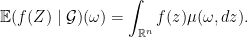
The above two actually comes from the existence of regular conditional distribution which is an important result in measure-theoretic probability theory.

Now take ${A=C}$ and ${f(Z) = Z}$ , we have for almost all ${\omega\in \Omega}$ ,

$\displaystyle \mathbb{E}(1_{\{Z\in C\}}\mid \mathcal{G})(\omega) = \int_{C} \mu(\omega, dz)$

and

$\displaystyle \mathbb{E}(Z\mid \mathcal{G}) (\omega)= \int_{\mathbb{R}^n} z \mu(\omega, dz).$

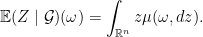
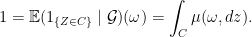
But since ${\mathop{\mathbb P}(Z\in C)=1}$ , we know that for almost all ${\omega \in \Omega}$ ,

$\displaystyle 1= \mathbb{E}(1_{\{Z\in C\}}\mid \mathcal{G})(\omega) = \int_{C} \mu(\omega, dz).$

Thus for almost all ${\omega}$ we have a probability distribution ${\mu(\omega, dz)}$ on ${{\mathbb R}^n}$ with mean equals to ${\mathop{\mathbb E} (Z\mid \mathcal{G} )(\omega)}$ and ${\int_C \mu (\omega ,dz) =1}$ . This is exactly the situation of Theorem 1. Thus by applying Theorem 1 to the probability measure ${\mu(\omega, dz)}$ , we find that