We consider global conditioning property of Linear Program (LP) here. Let’s first define the problem. The standard form of LP is
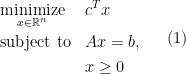
where 


Now suppose we add perturbation 


Let 


Such questions are called the conditioning of Program (2). It asks under some perturbation, how does the solution and optimal value changes accordingly. In general, we hope that Program (1) and (2) to be stable in the sense that small perturbation in the data, i.e., 


- Whether
- Whether
To address the first issue, we make our first assumption that
A1: Program (2) has a solution and the optimal value is finite.
Under A1, by strong duality of LP, we have that Program (1) also has a solution and the optimal value is the same as the optimal value of Program (2). This, in particular, implies that (1) is feasible. We now characterize the region where

the set of vertices of 


Now according to the Resolution Theorem of the primal polyhedron, we have

Using this representation, the fact that the primal of Program (3) is

and strong duality continue to hold for (3) and (5) as (5) is feasible by A1, the value of

Thus it is immediate that the region where

In particular, if 
To address the issue whether
A2: All the basic feasible solution of (1) are non-degenerate, i.e., all vertices of the feasible region of Program (1) have exactly 
Under this condition, and the definition of basic feasible solution, we know if 


is the unique solution to Program (3) where 

and
where 
By defining

which is a polyhedron, we may write the above compactly as

Then it is easy to see that the Lipschitz condition of

where 


Similarly, by using the theorem in this post, we see that

where 

Theorem 1 Recall
is the set of extreme points of the feasible region of (1),
is the set of extreme points of the feasible region of (1) and
. Under assumption A1 and A2, we have for all
,
and
where
are arbitrary norms. Here
.

How might one bound the Lipschitz constants

The former might be done by giving a bound of the diameter of the feasible region
 and a set of
  linear functions
  where each
  being closed polyhedrons in
  , i.e.,
  for some
  , and
, and  and
and  . Moreover, for any
  , and
, and  , we have
  . Then we can define function
  on
on  such that
 is convex. We now state a theorem concerning the Lipschitz constant of
  ,
,  -Lipschitz continuous with respect to
  and
and  , i.e., for all
  ,
, 
 is
is 
 ,
,  and
and  . we see the inequality
 for any
  , we have that there exists
  and corresponding
  such that
 where
where  . We also let
  and
and  . These
  s have the property that
 by
by
 is due to inequality
  is due to the definition of operator norm and
  is using equality
 and we know that
  only takes value in a convex set
  , i.e.,

 exists. It is then natural to ask how about conditional expectation. Is it true for any reasonable sigma-algebra
  that
that
 , and for any probability measure
  on
on  with
with
 to
to  is the usual Borel sigma algebra on
  . If
. If 

 .
. such that for almost all
  , we have for any

 , we have
 and
and  , we have for almost all
  ,
,
 , we know that for almost all
 we have a probability distribution
  on
on  with mean equals to
  and
and  . This is exactly the situation of Theorem
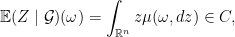
 ,
,  ,
,  where
where  and
and  are cumulative distribution function and
  are finite. We prove the following theorem.
 norm) For independent random variables

 .
. is usually referred as mean absolute difference and it measures the spread of a distribution. I don’t know the term for the quantity
  but what it measures is the difference between the distribution
  to estimate/predicts
  , then the expected error (the cross mean difference) in terms of absolute value (
 , which can be considered as variance and the difference in the two distribution ,i.e.,
  , which can be considered as bias.
 norm) and it is
 , and the difference of mean can be considered as bias as well.
 both have first finite moments. In the case either
  .
.

 and
and 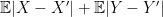 which is finite because
  is
is 
 . If
. If 

 ,
,

 .
. is very small, then how small is the distance
  . We might expect that
  will imply that
  . This is true if
  is compact and
  , and the distance to the solution, i.e.,
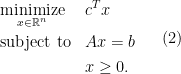
 .
.  means each coordinate of
  , and the distance to the solution set
  to be
to be  . Note that the norm here is arbitrary, not necessarily the Euclidean norm.
 which depends only on
  ,
,
 , and the distance to the solution set, i.e.
  , are the same up to a multiplicative constant. The right inequality of the theorem is usually referred to as linear growth in the optimization literature.
 where
where  and
and  for
for  and
and  . Here
  is the dual norm and
  are extreme points and extreme rays. We assume there are
  many extreme points and
  many extreme rays with first
  s and first
  are in the optimal set
  . See the proof for more detail.
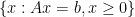 and
and 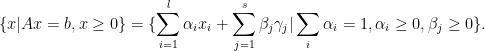
 s are extreme points of the feasible region and
  s are extreme rays. By scaling the extreme rays, we can assume that
  for all
  .
.
 many
many  and
and  since the
  .
.
 and
and  .
.
 for all
  here.
here. . We have
 and the inequality is because of the definition of
  and the
  s are positive.
 with
with  and
and  and apply triangular inequality to the above quantity, we have
 . The second inequality is applying the definition of
  and
and  . The first equality is due to
  and the second equality is due to
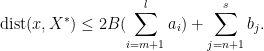
 by our previous argument, we see that setting


 , then
 is actually bounded and closed (
 .
. . We have
 and
and  are
are  such that


 and
and  where
where  or
or  is understood as
  and we overload the notation
  to mean
  . The probability space
  are convex sets in
  , then there exists a nonzero
  such that
 .
. is always an interval.
 dimension in
  for some
  and
and  .
. is not in
  such that
 almost surely, we should have
 , we see that
  with probability
  . Since intersection of the hyperplane of
  and
and  dimensional affine space.
 . After a proper translation and rotation, we can say that
  and we want to argue that the mean of
  , we should have its mean in the interval. If the interval is half open and half closed and if the means is not in the interval, then
  must be the open end of the interval since expectation preserves order, but this means that
  . This completes the proof.
  to a measurable space
  where each singleton set of
  is in
is in  . Let each
  be a real valued (Borel measurable) function with its domain to be
  . Given
 such that
  values in
 , then just ignore these. I put these term here just to make sure the that the theorem is rigorous enough.)
 with its first


 and
and  .
. and its all
  th order moments are finite, i.e.,
 . Each
  here is a nonnegative integer. The total number of moments in this case is
  . Then there is a real random vector
  such that it takes no more than
  values, and
 , and any random variable

 takes only finitely many value. But it is true that
 is
is
 which takes value only in
  , by Lemma
 has a FINITE representation in terms of
  s!
s! ,
,  and
and  such that
 for some
  , we can simply take the distribution of
 .
. 